Introduction
Gender differences in the labor market are prevalent, as the economic literature and the numerous reports by international institutions suggest. In a well-known meta-analysis, Weichselbaumer and Winter-Ebdmer (2005) estimate that even though the gap clo sed significantly between 1970 and today, differences still loom large. Women received hourly wages that, on average, are around 20% less than men. While this measure of differences in the labor market has been used, it provides only a rough estimate, a s it does not take into consideration the act that men and women could have different educational attainments, work in different occupations and industries and so on. Measures that account for these differences in characteristics paint a less optimistic picture. Conditional gender wage gap proved to be remarkably stable in the same period.
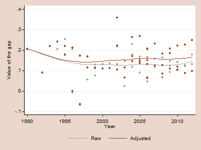
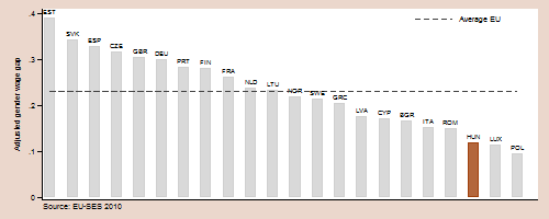
This report provides a summary of the measures of the gender wage gap over time. First, we describe the decomposition method used to recover the conditional wage gap. Then, we summarize the characteristics of the various sources of individual data avail able. Unlike previous research, we combine several databases in our analysis in order to maximize reliability of the results. Finally, we present the evolution of the gender wage gap for the country over time and a comparison to other economies from the EU.
Methods for analysis of gender wage gap
Several methods were developed to decompose the gender wage gap into a component attributable to differences in individual characteristics and into a component that cannot be explained by those characteristics. All these methods seek to identify how men and women differ in terms of observable characteristics (education, age, industry, ...) and account for these differences in wages. Whatever is left unexplained informs of the gender differences, usually referred to as the gender wage gap. This compon ent is often attributed to gender wage inequality or gender wage discrimination.
We follow the approach developed by Ñopo (2008) due to a number of advantages it offers. First, it is based on perfect matching, so the adjusted wage gap is estimated only among the comparable workers. Second, it requires no assumption about the relatio nship between wages and individual characteristics. Finally, Goraus et al (2017) demonstrate that estimates from Ñopo decomposition are less sensitive to the omission of variables. Often important information concerning either firm characteristics or ho usehold characteristics are missing in the data, which could bias estimates from other methods.
Sources
We collect a wide array of data sources with information about individuals. While the use of a broader set of databases has the advantage of a better coverage, both across countries and years, these databases are not fully comparable. Being constructed for different purposes, each of them has advantages and disadvantages. Below we provide a summary of the main characteristics of each database with a link to the website.
It is a household budget survey conducted in Member States. In principle it contains high quality data on both household structure and earnings, but some relevant data are missing. This survey was conducted between 1994 and 2001 and was subsequently sup erseded by the Survey on Income and Living Conditions in 2003. Unfortunately, EU-SILC only provides information on annual labour earnings, which limits the scope of comparison to workers with full-year full-time positions.
It is worldwide initiative to collect data for social sciences research. Though the focus is on the study of attitudes and behaviours, the ISSP also collects information useful for the estimation of the gender wage gap, as wages and hours worked and hou sehold level data. Moreover, and unlike alternative official sources, these data were collected in transition countries since the early 1990's and are available free of charge. Possible shortcomings refer to sample size (usually less than two thousand o bservations) and to the coding of wages, i.e. in some particular countries and years wages are interval coded, which prevents the estimation of the gender wage gap. Nevertheless, the use of ISSP is not uncommon in international comparisons, see .
Developed by The World Bank, LSMS is a standardized a household budget survey that provides wide array of information on household and individual characteristics. The survey is usually implemented by statistical offices from the beneficiary countries, w hich might raise some doubts on both the quality of the data (e.g.a large proportion of missing values) and representativeness of the sample. LSMS more than compensates for this potential pitfalls with its sample size, which lays between 10 000 and 30 0 00 observations. Even though LSMS data are gathered from around the world, the current analysis employs databases from Albania, Azerbaijan, Bosnia, Bulgaria, Kyrgyzstan, Serbia and Tajikistan.
Given the focus on labor market phenomena, these survey allow to tackle a potentially wider array of issues, including overtime and self-employment. Moreover, information on wages tends to be more precise, and quite often it allows to recover both gross and net payments. However, without access to household roster, accounting for the household structure is impossible, which prevents taking good account of asymmetric labor supply decisions by men and women in the presence of small children in the house hold. Finally, these databases are usually large, with around 100 000 respondents per country.
Unlike previous sources, SES is collected from employers, which results on more precise information on workers' characteristics, as well as wages and hours worked. The SES is collected regularly in all European countries, though each country has its own provisions in terms of sample coverage (e.g. the inclusion of public administration and of firms with less than ten employees is optional) and number of employees interviewed within each firm. In terms of sample size, they can be well above the 100 000 particularly in the case of large countries. These databases have two shortcomings for the analysis of the gender wage gaps. First, they lack information on the household structure. Second, sample is restricted to employees. Together, these shortcoming s prevent any analysis of decisions to participate into the labor market.
For Hungary, the following data sources are available:
1.ISSP
2.Life in Transition Survey (2006)
3.Structure of earnings survey
4.Survey on Income and Living Conditions (EU)
Results for Hungary
Figure 1 : Evolution of the gender wage gap over time

Figure 2 : Gender wage gap against other to EU countries

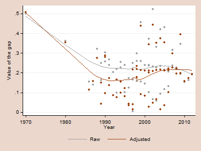
Figure 3: Evolution of the gender employment gap over time

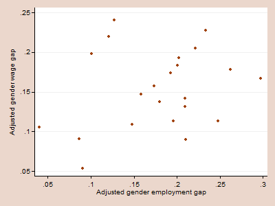
Figure 4: Comparison of the employment and wage gaps

Databases used in the estimation of the gender gaps in Hungary
| Year | -- | Gender Wage Gaps | -- | -- | Gender Employment Gaps | -- |
|---|---|---|---|---|---|---|
| -- | Sources | Raw gap | Adjusted gap | Sources | Raw gap | Adjusted gap |
| 1970 | . | . | IPUMS | 0.50 | 0.51 | |
| 1980 | . | . | IPUMS | 0.36 | 0.35 | |
| 1986 | . | . | ISSP | 0.16 | 0.11 | |
| 1987 | . | . | ISSP | 0.14 | 0.16 | |
| 1988 | . | . | ISSP | 0.32 | 0.28 | |
| 1989 | . | . | ISSP, LITS | 0.21 | 0.10 | |
| 1990 | ISSP | 0.21 | 0.20 | ISSP, IPUMS, LITS | 0.29 | 0.22 |
| 1991 | . | . | ISSP, LITS | 0.25 | 0.16 | |
| 1992 | ISSP | 0.09 | 0.09 | LITS | 0.20 | 0.09 |
| 1993 | ISSP | 0.22 | 0.22 | ISSP, LITS | 0.16 | 0.12 |
| 1994 | ISSP | 0.20 | 0.24 | ISSP, LITS | 0.24 | 0.13 |
| 1995 | ISSP, SES | 0.22 | 0.20 | ISSP, LITS | 0.17 | 0.10 |
| 1996 | ISSP, SES | 0.10 | 0.10 | ISSP, LITS | 0.15 | 0.04 |
| 1997 | ISSP, SES | 0.05 | 0.05 | ISSP, LFS, LITS | 0.14 | 0.09 |
| 1998 | ISSP, SES | 0.11 | 0.14 | ISSP, LFS, LITS | 0.24 | 0.21 |
| 1999 | ISSP, SES | 0.10 | 0.11 | ISSP, LFS, LITS | 0.29 | 0.25 |
| 2000 | SES | 0.13 | 0.11 | LFS, LITS | 0.19 | 0.15 |
| 2001 | SES | 0.14 | 0.11 | ISSP, IPUMS, LFS, LITS | 0.24 | 0.20 |
| 2002 | ISSP, SES | 0.16 | 0.23 | ISSP, LFS, LITS | 0.27 | 0.23 |
| 2003 | ISSP, SES | 0.09 | 0.09 | ISSP, LFS, LITS | 0.20 | 0.21 |
| 2004 | ISSP, SES, SILC | 0.17 | 0.19 | ISSP, LFS, LITS | 0.25 | 0.20 |
| 2005 | ISSP, SES, SILC | 0.14 | 0.18 | ISSP, LFS, LITS | 0.25 | 0.20 |
| 2006 | ISSP, SES, SILC | 0.12 | 0.14 | ISSP, LFS, LITS | 0.19 | 0.18 |
| 2007 | SES, SILC | 0.14 | 0.18 | ISSP, LFS | 0.28 | 0.26 |
| 2008 | ISSP, SES, SILC | 0.10 | 0.13 | ISSP, LFS | 0.22 | 0.21 |
| 2009 | ISSP, SES, SILC | 0.12 | 0.17 | ISSP, LFS | 0.27 | 0.30 |
| 2010 | SES, SILC | 0.13 | 0.15 | LFS | 0.15 | 0.16 |
| 2011 | SES, SILC | 0.12 | 0.16 | LFS | 0.16 | 0.17 |
| 2012 | SES, SILC | 0.16 | 0.17 | LFS | 0.19 | 0.19 |
References
Goraus, K., J. Tyrowicz and L. van der Velde (2017) Which gender wage gap estimate to trust? A comparative analysis. Review of Income and Wealth, Vol. 63, No. 1, pp.: 118-146. Link
Ñopo, H. (2008) Matching as a tool to decompose wage gaps. Review of Economics and Statistics, Vol. 90, No. 2, pp.: 290-299. Link
Weichselbaumer, D. and Winter-Ebmer, R. (2005), A meta-analysis of the international gender wage gap. Journal of Economic Surveys, Vol. 19, No. 3, pp.: 479-511. Link
